Variational Monte Carlo

This is the fourth part in a short series of blog posts about quantum Monte Carlo (QMC). The series is derived from an introductory lecture I gave on the subject at the University of Guelph.

Part 1 – calculating Pi with Monte Carlo

Part 2 – Galton’s peg board and the central limit theorem

Part 3 – Markov Chain Monte Carlo

Introduction to QMC – Part 4: High dimensional calculations with VMC

In the previous post, Markov Chains were introduced along with the Metropolis algorithm. We then looked at a Markov Chain Monte Carlo (MCMC) Python script for sampling probability distributions. Today we’ll use a modified version of that script to perform calculations inspired by quantum mechanics. This will involve sampling high dimensional probability distributions for systems with multiple particles.

We are heading into complicated territory, so I set up the first section of this post in question-answer format.

 

Why is it called VMC and not MCMC?

As far as I can tell, variational Monte Carlo (VMC) is the same as MCMC. The name was probably inspired by the variational theorem from quantum mechanics, but we’ll get to this later. For now let’s simply pose the problem:

Given a probability distribution , where is the configuration vector for the positions of particles in a box, calculate the average energy of the system.

Why do we need to worry about probability distributions? Because in the quantum world things to not always have well defined positions, but instead only have well defined probabilities of being in specific positions. Hence the existence of probability distributions.

 

What function are we calculating?

We’ll calculate the average value of the local energy , which is defined as the sum of kinetic and potential energies:

It’s not unreasonable to plug in some and calculate by hand or with a computer, but to calculate the average we’ll need to sample the probability distribution with Monte Carlo.

Kinetic term T

The kinetic energy will depend on the second derivative of the wave function, which is relatively difficult and computationally time consuming to calculate. To avoid dealing with this beast we’ll use a made-up function

It could be interpreted as the particles having more kinetic energy (i.e., larger ) depending on how far they are from the center of the box (as we’ll see the box is centered about r=(0,0)). This doesn’t make sense physically of course.

Potential term V

This is the cumulative potential energy of the particles, and unlike it will be calculated “for real” (i.e., how it actually can be done in practice). We’ll assume the system is split into equal sized groups of different “species” particles, denoted and [1], and only consider interactions between particles of different species. In this case we have

where is the two-body potential and is the distance between particles and . The notation ensures that we only count each interaction once. We'll take to be a shifted Gaussian:

from scipy import stats
mu = 0.5
sig = 0.1
y = lambda r: -stats.norm.pdf((r-mu)/(sig))

We’ll focus on the case where , for which the potential becomes

 

What probability distribution will we sample?

From elementary quantum mechanics, the probability density is given by the square of the wave function. So, for our many-body wave function , we have that

The absolute value is meaningful when the wave function has imaginary components, which is not the case for us today. Our first will be a linear combination of single-particle wave functions and [2]:

def prob_density(R, N):
    ''' The square of the many body wave function
        Psi_V(R). '''

    # e.g. for N=4:
    # psi_v = psi(r_1) + psi(r_2) + psi(r_3) + psi(r_4)
    psi_v = sum([psi_1(R[n][0], R[n][1]) for n in range(N)]) + \
            sum([psi_2(R[n][0], R[n][1]) for n in range(N)])

    # Setting anything outside the box equal to zero
    # This will keep particles inside
    for coordinate in R.ravel():
        if abs(coordinate) >= 1:
            psi_v = 0

    return np.float64(psi_v**2)

Our configuration space is two dimensional (so we can visualize it nicely) and so particle positions consist of just and coordinates, i.e. . Lets take to be a positive Gaussian and to be a negative Gaussian.

def psi_1(x, y):
    ''' A single-particle wave function. '''
    g1 = lambda x, y: mlab.bivariate_normal(x, y, 0.2, 0.2, -0.25, -0.25, 0)
    return g1(x, y)

def psi_2(x, y):
    ''' A single-particle wave function. '''
    g2 = lambda x, y: -mlab.bivariate_normal(x, y, 0.2, 0.2, 0.25, 0.25, 0)
    return g2(x, y)

The summation of and looks like:

If we take this summation to be the wave function of a system with just one particle then the associated probability distribution for the particle location would look like:

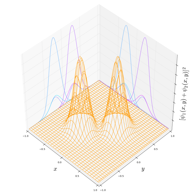
So what about a plot of the many-body wave function ? We would require a higher dimensional space for this. Take the example of particles. In this case we have and would need to include an axes for not just “ and ” as done above, but for , , , , , , , and .

 

Calculating the average energy

We’ll focus on the particle system where 2 are species and 2 are species . The wave function in this case is

Running a quick simulation with 1000 walkers (i.e., 1000 samples per step) for 40 steps, the samples look like this:

The top left panel shows the initial state where walkers are distributed randomly. As the system equilibrates we see them drifting into areas where the probability density is large. Species is plotted in blue and in red.

To calculate we average over many values of for equilibrated samples. An example using 200 walkers is shown below.

Each point is an average over all walkers at the given step. In this case we calculate an average energy of 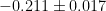, where the first 200 steps have been excluded so we only average over the equilibrated system. The error, as shown by the red band around the average, is calculated as the sample standard deviation of [3]:

Running a calculation with 2000 walkers, we can see a dramatically reduced error:

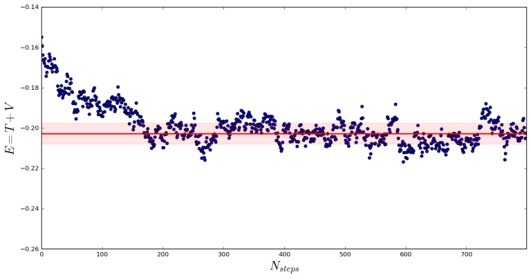
Now we calculate , which agrees within error to the previous calculation.

 

Equilibration times

In the calculations above, the system appeared to equilibrate almost immediately. This is because the initial configurations were randomly distributed about the box. If instead we force the particles to start near the corners of the box (far away from the areas where the probability distribution is large) we can clearly see decreasing as equilibration occurs. Below we plot this along with the particle density from various regions of the calculation (as marked in yellow in the right panel).

 

Variational Theorem

The usefulness of VMC for quantum mechanical problems has to do with the variational theorem. In words, this theorem says that the energy expectation value (denoted for short) is minimized by the true ground state wave function of the system. This can be written mathematically as follows:

where is the ground state energy of the system. A proof can be found at the bottom of page 60 of my masters thesis. The triple-bar equals sign simply means “is defined as”, what’s important is the other part of the equation.

If the name of the game is to find the ground state energy, which is often the case, then a good estimate can be achieved using VMC. A can include variable parameters to optimize, which is done by calculating for a particular set of parameters (the same way we’ve calcualted in this post) and repeating for different parameters until the lowest value is found. The resulting energy estimate will be an upper bound to the true ground state energy of the system.

 

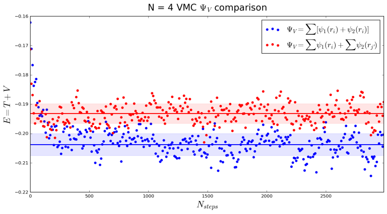
Calculating average energy with a different many-body wave function

To show how changing can impact the calculation of we’ll adjust the wave function:

where the two species and now have different single-particle wave functions. As shown above, we define as the left Gaussian (looking back to the first figure) and as the right one. For we now have:

The new probability density will be:

def prob_density(R, N):
    ''' The square of the many body wave function
        Psi_V(R). '''

    psi_v = sum([psi_1(R[n][0], R[n][1]) for n in range(int(N/2))]) + \
            sum([psi_2(R[n][0], R[n][1]) for n in range(int(N/2),N)])

    # Setting anything outside the box equal to zero
    # This will keep particles inside
    for coordinate in R.ravel():
        if abs(coordinate) >= 1:
            psi_v = 0

    return np.float64(psi_v**2)

This should have the effect of separating the two species of particles. Do you think will become larger or smaller as a result?

Plotting some of the samples, we can see how the system now equilibrates according to the new probability density:

Comparing a calculation with the new (red) to the old one (blue), we see an increase in :

 

Thanks for reading! You can find the entire ipython notebook document here. If you would like to discuss any of the plots or have any questions or corrections, please write a comment. You are also welcome to email me at agalea91@gmail.com or tweet me @agalea91

 

 

[1] – For example we could have a system of cold atoms with two species that are identical except for the total spin. Where one species is spin-up and the other is spin-down.

[2] – I made the many-body wave function a sum of single-particle wavefunctions but it would have been more realistic to make it a product of ‘s as can be seen here (for example).

[3] – In practice, the error on Monte Carlo calculations is often given by the standard deviation divided by . Otherwise the error does not decrease as increases, which should intuitively be the case because we are building confidence in the calculation as the simulation is run longer. For more information see this article – specifically the first few equations and Figure 1.