Top 20 Pandas, NumPy and SciPy functions on GitHub

A few months ago I noticed a blog post listing the most commonly used functions/modules for a few of the most popular python libraries as determined by number of instances on Github. I’ve created visualizations of these results and wrote examples for the top 10 from each library. A few are included here, but the full set of examples can be found in the ipython notebook file.

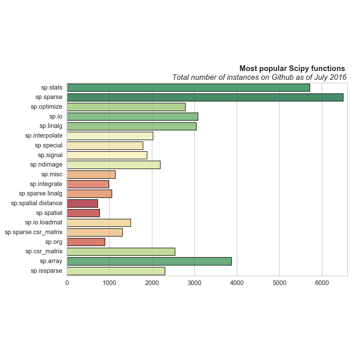
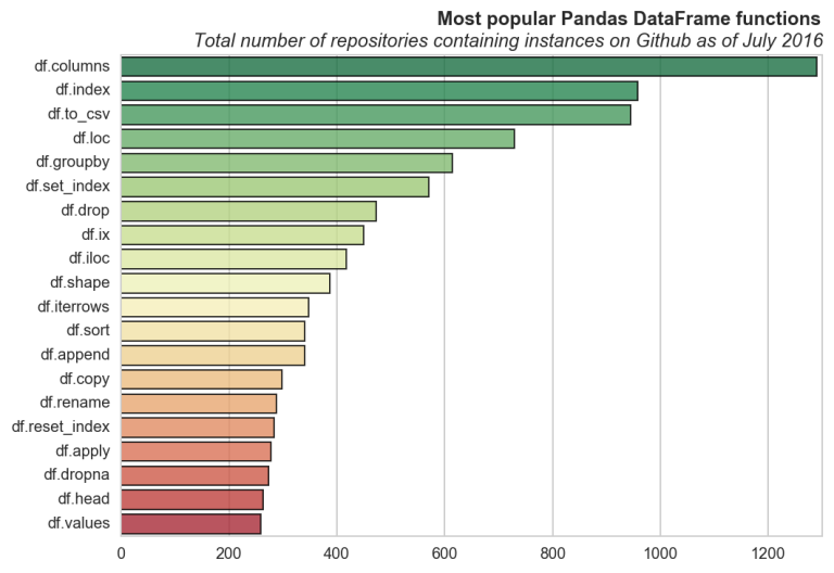
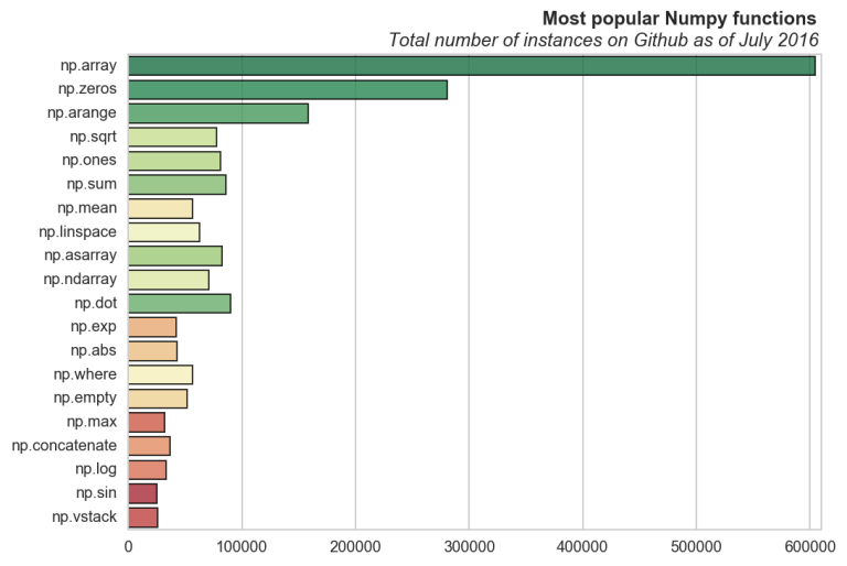
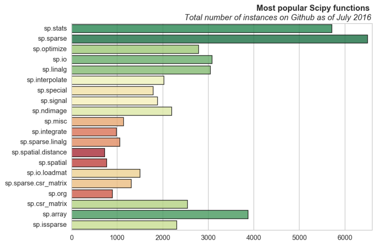
Most popular Pandas, Pandas.DataFrame, NumPy, and SciPy functions on Github

I pulled the statistics from the original post (linked to above) using requests and BeautifulSoup for python. The bar plots were made with matplotlib and seaborn, where the functions are ordered by the number of unique repositories containing instances. For example we see that pd.Timestamp is not as often used in a project as a number of others, despite it having a very high number of total instances on Github.

Pandas

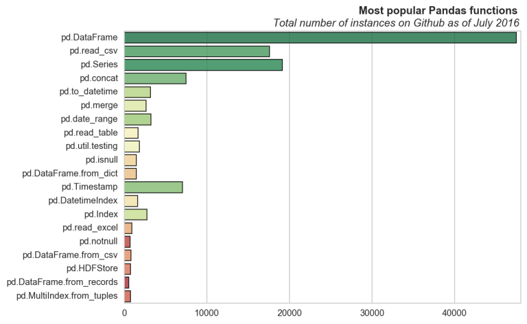
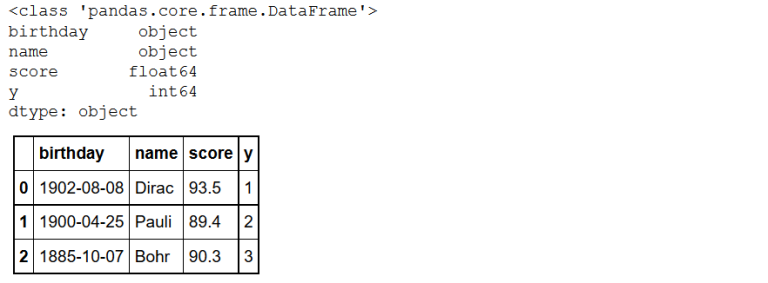
1) Dataframe: Creates a dataframe object.

df = pd.DataFrame(data={'y': [1, 2, 3],
                        'score': [93.5, 89.4, 90.3],
                        'name': ['Dirac', 'Pauli', 'Bohr'],
                        'birthday': ['1902-08-08', '1900-04-25', '1885-10-07']})
print(type(df))
print(df.dtypes)
df

 

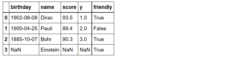
6) Merge: Combine dataframes.

df_new = pd.DataFrame(data=list(zip(['Dirac', 'Pauli', 'Bohr', 'Einstein'],
                                    [True, False, True, True])),
                      columns=['name', 'friendly'])

df_merge = pd.merge(left=df, right=df_new, on='name', how='outer')
df_merge

 

NumPy

 

3) arange: Create an array of evenly spaced values between two limits.

np.arange(start=1.5, stop=8.5, step=0.7, dtype=float)

 

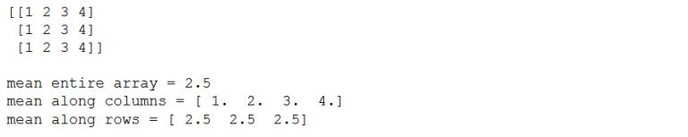
8) mean: Get mean of all values in list/array or along rows or columns.

vals = np.array([1, 2, 3, 4]*3).reshape((3, 4))
print(vals)
print('')
print('mean entire array =', np.mean(vals))
print('mean along columns =', np.mean(vals, axis=0))
print('mean along rows =', np.mean(vals, axis=1))

 

SciPy

 

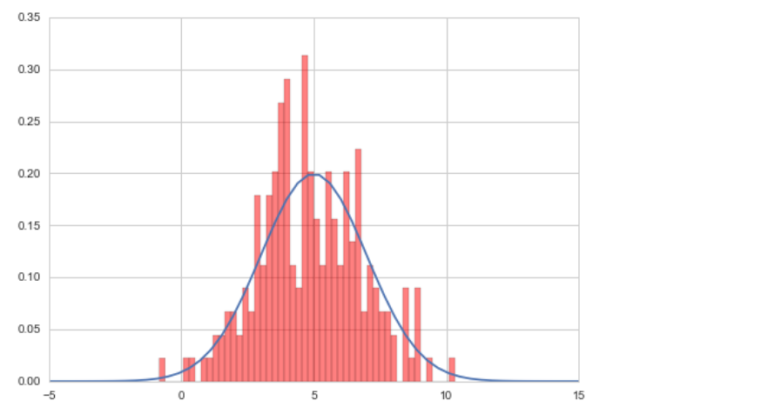
1) stats: A module containing various statistical functions and distributions (continuous and discrete).

# Normal distribution:

# plot Gaussian
x = np.linspace(-5,15,50)
plt.plot(x, sp.stats.norm.pdf(x=x, loc=5, scale=2))

# plot histogram of randomly sampling
np.random.seed(3)
plt.hist(sp.stats.norm.rvs(loc=5, scale=2, size=200),
                           bins=50, normed=True, color='red', alpha=0.5)
plt.show()

 

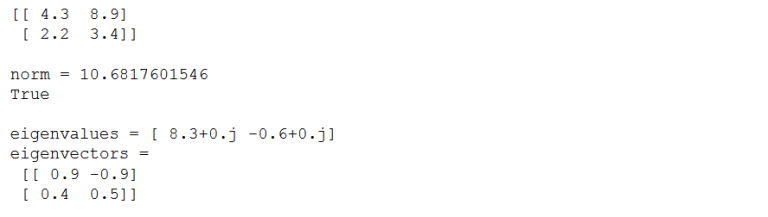
5) linalg: Among other things, this module contains linear algebra functions including inverse (linalg.inv), determinant (linalg.det), and matrix/vector norm (linalg.norm) along with eigenvalue tools e.g., linalg.eig.

matrix = np.array([[4.3, 8.9],[2.2, 3.4]])
print(matrix)
print('')

# Find norm
norm = sp.linalg.norm(matrix)
print('norm =', norm)
# Alternate method
print(norm == np.square([v for row in matrix for v in row]).sum()**(0.5))
print('')

# Get eigenvalues and eigenvectors
eigvals, eigvecs = sp.linalg.eig(matrix)
print('eigenvalues =', eigvals)
print('eigenvectors =\n', eigvecs)

 

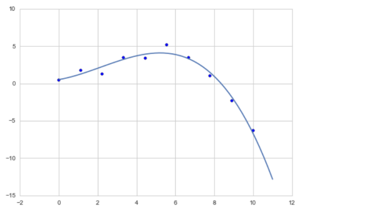
6) interpolate: A module containing splines and other interpolation tools.

# Spline fit for scattered points

x = np.linspace(0, 10, 10)
xs = np.linspace(0, 11, 50)
y = np.array([0.5, 1.8, 1.3, 3.5, 3.4,
5.2, 3.5, 1.0, -2.3, -6.3])
spline = sp.interpolate.UnivariateSpline(x, y)
plt.scatter(x, y); plt.plot(xs, spline(xs))
plt.show()

 

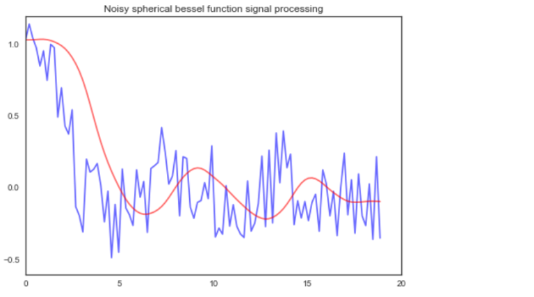
8) signal: This module must be import directly. It contains tools for signal processing.

# Fit noisy signal smooth line
import scipy.signal
np.random.seed(0)

# Create noisy data
x = np.linspace(0,6*np.pi,100)
y = [sp.special.sph_jn(n=3, z=xi)[0][0] for xi in x]
y = [yi + (np.random.random()-0.5)*0.7 for yi in y]
# y = np.sin(x)

# Get paramters for an order 3 lowpass butterworth filter
b, a = sp.signal.butter(3, 0.08)

# Initialize filter
zi = sp.signal.lfilter_zi(b, a)

# Apply filter
y_smooth, _ = sp.signal.lfilter(b, a, y, zi=zi*y[0])

plt.plot(x, y, c='blue', alpha=0.6)
plt.plot(x, y_smooth, c='red', alpha=0.6)
plt.title('Noisy spherical bessel function signal processing')
plt.savefig('noisy_signal_fit.png', bbox_inches='tight')
plt.show()

 

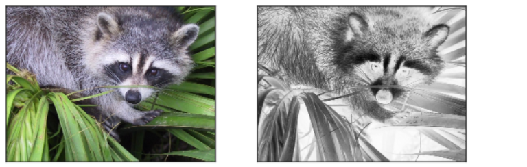
10) misc: A module containing “utilities that don’t have another home”. Based on the google search results, people often use `misc.imread` and `mics.imsave` to open and save pictures.

# Get a raccoon face

# Get the raccoon
pics = sp.misc.face(), sp.misc.face(gray=True)

# Look at it
fig, axes = plt.subplots(1, 2, figsize=(10, 4))
for pic, ax in zip(pics, axes):
    ax.imshow(pic); ax.set_xticks([]); ax.set_yticks([])
plt.show()

 

 

 

Thanks for reading. As mentioned earlier, you can see a full list of examples in my ipython notebook. I would like to acknowledge Robert for mining the usage data from Github, here is a link to his blog.

If you would like to discuss anything or have questions/corrections then please write a comment, email me at agalea91@gmail.com, or tweet me @agalea91